|
|
You are here: GSI Wiki>FIRST Web>ReconstructionSoftware>SimulationSoftware (2012-10-30, AlessioSarti)Edit Attach

Simulation Software
This is the home page of the simulation software for the FIRST Experiment. You can find details on the simulation code, event samples produced by the simulation, and instructions to access and run to the simulation code here.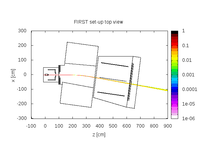
- Simulation Software
Presentations / Documentation
- Talk at Software meeting Jan 2011
General structure of the simulation
The simulation of the whole FIRST Experiment set-up is done with the Monte Carlo code FLUKA.- Input: Geometry and material input files for FLUKA are generated via C/C++-based files.
- Output: All physical and detector-related output quantities are written and stored in a ROOT-file (C++) for further analysis.
- For each event, tracks of all produced hadronic particles in the FIRST geometry are saved in ROOT file in the
Track block.- i.e.: fixed particle properties, initial/final position, momentum, parent particle, etc.
- Basic detector-related quantities are also saved in the same ROOT file in the
Subdetector blocks.- i.e.: (quenched) energy depositions in sensitive regions, entrance/exit position, momentum, arrival time, particle ID, etc.
- The basic detector-related quantities are converted to signals (adding noise and uncertainties) and digitized and are also saved in the same ROOT file in the
Subdetector blocks.- i.e.: TOF-Wall & Start Counter: scintillator light yield and arrival time, Vertex detector: Simulating cluster of activated pixel for each passing particle with simple model
- No EM particle tracks are currently scored at the moment (can be easily switched on, but lots of data!)
- The energy depositions by EM particles in sensitive regions are associated with the parent hadronic particles.
- No delta rays are produced at the moment in most of the geometry to save computation time.
Simulation Code
How to get event data sets: A list of standard event data sets can be found in the next section. In near future these data sets will be available for download at a central - for the moment please ask. If needed, further sets can be generated by running the simulation code yourself or on demand. How to get the simulation code: The SVN repository with the general Monte Carlo simulation of FIRST is currently available at GSI. See the Reconstruction Software page for instructions. How to install and run: The simulations uses the Monte Carlo code FLUKA, including the rQMD and BME model. The BME model is only needed if accurate prediction of non-elastic interactions below 100MeV/n is of importance (but now included in the FLUKA2011 release). Further the simulation is using ROOT. Once these programs are installed you should be able to compile and run the simulation with the following steps:- cd FIRST/sim/trunk
- source lib_setup.csh
- ./runstp
- ./runtest
Currently available datasets and relative conditions
The events are kept under- lustre: /lustre/bio/first/MC_production
- s371 scratch area: /s/s371/MC_prod
| ID | root-file | aux-files | No. of events | Creation date | Availability |
General description |
|---|---|---|---|---|---|---|
| 039 | MC_ID039_Evt1k.root (1k) MC_ID039_Evt100k.root (100k) | MC_ID039.tar.gz | 1k/100k | 01.04.2011 | dito | Full FIRST events, commit 039 |
| 040 | MC_ID040_Evt1k.root (1k) MC_ID040_Evt100k.root (100k) | MC_ID040.tar.gz | 1k/100k | 20.04.2011 | dito | Full FIRST events, commit 041 |
| 042 | MC_ID042_Evt1k.root (1k) MC_ID042_Evt100k.root (100k) | MC_ID042.tar.gz | 1k/100k | 09.05.2011 | dito | Full FIRST events, commit 042 |
| 043 | MC_ID043_Evt1k.root (1k) MC_ID043_Evt100k.root (100k) | MC_ID043.tar.gz | 1k/100k | 17.06.2011 | dito | Full FIRST events, commit 043 |
| 044 | MC_ID044_Evt1k.root (1k) MC_ID044_Evt100k.root (100k) | MC_ID044.tar.gz | 1k/100k | 20.07.2011 | dito | Full FIRST events, commit 044 |
| 046 | MC_ID046_Evt1k.root (1k) MC_ID046_Evt100k.root (100k) | MC_ID046.tar.gz | 1k/100k | 08.11.2011 | dito | Full FIRST events, commit 046 |
| 050 | carbonTG_v50 (100k) vacuumTG_v50 (1k) | same flag as root file | 1k/100k | 15.07.2012 | lustre,s371 | fixed vtx positioning/decoding |
| 051 | carbonTG_v51 (100k) | same flag as root file | 100k | 26.07.2012 | lustre,s371 | implemented vtx tilt[ wrong sign ]/shift[ too much ] (still hardcoded) |
| 052 | carbonTG_v52 (100k) | same flag as root file | 100k | 4.08.2012 | lustre,s371 | implemented proper vtx tilt/shift. Target TOO wide, misplaced. Software version: tag 731 |
| 053 | carbonTG_v53 (100k) | same flag as root file | 100k | 7.08.2012 | lustre,s371 | Fixed target position/dimension. Software version: tag 747 |
| 055 | carbonTG_v55 (100k) | same flag as root file | 1k,100k | 29.10.2012 | lustre,s371 | Fixed ToF simulation, geometry. Software version: tag 966 |
| 056 | carbonTG_v56 (100k) | same flag as root file | 1k,100k | 20.10.2012 | lustre,s371 | Fixed BM resolution. Software version: tag 966 |
Log with Changes
Output of the simulation for reconstruction
In the following the naming scheme and content of the variables output to the ROOT-file are described. To access the information stored in the root-file easily you can use the Evento-class (under FIRST/sim/trunk).// GENERAL SYNTAX FOR DETECTOR VARIABLES // tr...: Track // st...: MAGARITA start counter // tg...: Target // mi...: MIMOSA 26 vertex tracker // ke...: KENTROS // mu...: TP-MUSIC IV // tw...: TOF-Wall // on...: ONION veto detector // variables with raw Monte Carlo data // ...n: number of particles entering the sensitive region for this event // ...id: index of particle in "track common" // ...reg: sensitive region ID // ...inx,y,z: position where particles enters the sensitive region [cm] // ...outx,y,z: position where particles exits the sensitive region [cm] // ...inpx,py,pz: momentum when particles enters the sensitive region [GeV/c] // ...outpx,py,pz: momentum when particles exits the sensitive region [GeV/c] // ...de: energy deposition in sensitive region [GeV/cm^3] // ...al: quenched energy deposition in sensitive region (with Birk's law) [GeV/cm^3] // ...tim: time when particle enters the sensitive region [s] // ...Sig...: signal variables // ...Amp...: amplitude of signal // ...Time...: time of signal // ...Dig...: Digitized
Track block
  Int_t trn; //number of tracks for current event
  Int_t trid[MAXTR]; //generation number of the track (FLUKA intern number)
  Int_t trpaid[MAXTR]; //generation number of the track parent (FLUKA intern)
  Int_t trtype[MAXTR]; //particle type (FLUKA encoding, see below)
  Double_t trmass[MAXTR]; // particles mass [GeVc^2]
  Int_t trcha[MAXTR]; //charge of particle
  Int_t trbar[MAXTR]; //barionic number
  Int_t trreg[MAXTR]; //production region of particle (FLUKA region number, for decoding can be done with the corresponding out-file)
  Int_t trgen[MAXTR]; //type of generation interaction (FLUKA encoding, see FLUKA file: mgdraw.f)
  Int_t trdead[MAXTR]; // with which interaction the particle dies (FLUKA encoding, see FLUKA file: mgdraw.f)
  Double_t tritime[MAXTR];//production time of the track
  Double_t trix[MAXTR]; //track initial position [cm]
  Double_t triy[MAXTR];
  Double_t triz[MAXTR];
  Double_t trfx[MAXTR]; //track final position [cm]
  Double_t trfy[MAXTR];
  Double_t trfz[MAXTR];
  Double_t tripx[MAXTR]; //track initial momentum [GeV/c]
  Double_t tripy[MAXTR];
  Double_t tripz[MAXTR];
  Double_t trpapx[MAXTR];//momentum of parent particle at production [GeV/c]
  Double_t trpapy[MAXTR];
  Double_t trpapz[MAXTR];
- Example: To look up for a give particle ID (..id[i]) from a detector block (e.g. keid[i]) the particle properties from the track block, one can retrieve them by tr...[(int)..id[i]-1] (e.g. trtype[(int)keid[i]-1]). Note the "-1"! (Comes from conversion of arrays from FORTRAN to C.)
- FLUKA encoding for particle types
- trfx,y,z: if this is (0,0,0) and also trdead=0 it usually means that the particle escaped the world without dying
- AnaTEST.py.txt: Example script reading the simulation root-file with pyROOT
Start Counter (Magarita) block
  Int_t stn; //number particles entering the start counter for current event
  Int_t stid[MAXST];
  Int_t stflg[MAXST];
  Double_t stinx[MAXST];
  Double_t stiny[MAXST];
  Double_t stinz[MAXST];
  Double_t stoutx[MAXST];
  Double_t stouty[MAXST];
  Double_t stoutz[MAXST];
  Double_t stinpx[MAXST];
  Double_t stinpy[MAXST];
  Double_t stinpz[MAXST];
  Double_t stoutpx[MAXST];
  Double_t stoutpy[MAXST];
  Double_t stoutpz[MAXST];
  Double_t stde[MAXST];
  Double_t stal[MAXST];
  Double_t sttim[MAXST];
//signal
  Double_t stSigAmp; //signal amplitude (\propto quenched energy deposition per event)
  Double_t stSigTime; //signal time (time from the starting of the primary particle)
  Int_t    stSigAmpDig; //as above but rescaled and converted to int values
  Int_t    stSigTimeDig;//as above but rescaled and converted to int values
Beam Monitor block
  Int_t nmon; //number particles entering the beam monitor for current event
  Int_t idmon[MAXMON];
  Int_t iview[MAXMON];
  Int_t icell[MAXMON];
  Int_t ilayer[MAXMON];
  Double_t xcamon[MAXMON];
  Double_t ycamon[MAXMON];
  Double_t zcamon[MAXMON];
  Double_t pxcamon[MAXMON];
  Double_t pycamon[MAXMON];
  Double_t pzcamon[MAXMON];
  Double_t rdrift[MAXMON];
  Double_t tdrift[MAXMON];
  Double_t timmon[MAXMON];
Target block
  Int_t tgn;
  Int_t tgid[MAXTG];
  Int_t tgflg[MAXTG];
  Double_t tginx[MAXTG];
  Double_t tginy[MAXTG];
  Double_t tginz[MAXTG];
  Double_t tgoutx[MAXTG];
  Double_t tgouty[MAXTG];
  Double_t tgoutz[MAXTG];
  Double_t tginpx[MAXTG];
  Double_t tginpy[MAXTG];
  Double_t tginpz[MAXTG];
  Double_t tgoutpx[MAXTG];
  Double_t tgoutpy[MAXTG];
  Double_t tgoutpz[MAXTG];
  Double_t tgtim[MAXTG];
Vertex (MIMOSA 26) Block
  //in this part we score for each pixel with ID miid all the tracks releasing energy in the pixel
  Int_t    min;
  Int_t    miid[MAXMI];
  Int_t    michip[MAXMI];
  Int_t    mincol[MAXMI];
  Int_t    minrow[MAXMI];
  Double_t mix[MAXMI];
  Double_t miy[MAXMI];
  Double_t miz[MAXMI];
  Double_t mipx[MAXMI];
  Double_t mipy[MAXMI];
  Double_t mipz[MAXMI];
  Double_t mide[MAXMI];
  Double_t mitim[MAXMI];
  //signal of MIMOSA26 (all the activated maps)
  Int_t    miSigN;
  Int_t    miSigChip[MAXMISIG]; //chipnumber
  Int_t    miSigIndex[MAXMISIG]; //pixel index in the chip
  Int_t    miSigCol[MAXMISIG]; //column
  Int_t    miSigRow[MAXMISIG]; //row
  Int_t    miSigId[MAXMISIG]; //particle ID in particle_common
  Double_t miSigTim[MAXMISIG]; //time when pixel activated
  Double_t miSigX[MAXMISIG]; //(global) coordinates of pixel
  Double_t miSigY[MAXMISIG]; //(global) coordinates of pixel
  Double_t miSigZ[MAXMISIG]; //(global) coordinates of pixel
  Double_t miSigPedest[MAXMISIG]; //pedestal on pixel
KENTROS block
  Int_t ken;
  Int_t keid[MAXKE];
  Int_t kereg[MAXKE];
  Int_t keregtype[MAXKE];//type of the detector segment barrel(=1), fiber(=2), small endcap(=3), big endcap(=4)
  Double_t keinx[MAXKE];
  Double_t keiny[MAXKE];
  Double_t keinz[MAXKE];
  Double_t keoutx[MAXKE];
  Double_t keouty[MAXKE];
  Double_t keoutz[MAXKE];
  Double_t keinpx[MAXKE];
  Double_t keinpy[MAXKE];
  Double_t keinpz[MAXKE];
  Double_t keoutpx[MAXKE];
  Double_t keoutpy[MAXKE];
  Double_t keoutpz[MAXKE];
  Double_t kede[MAXKE];
  Double_t keal[MAXKE];
  Double_t ketim[MAXKE];
//signal
  Int_t    keSigN;
  Int_t    keSigID[MAXKE];
  Double_t keSigTim[MAXKE];
  Double_t keSigAmp[MAXKE];
//digitised signal
  Int_t keSigDigN;
  Int_t keSigIDDig[MAXKE];
  Int_t keSigTimDig[MAXKE];
  Int_t keSigAmpDig[MAXKE];
TP-MUSIC IV block
  //MU_PRO_Nb= number of proporional chamber regions (=8)
  Int_t mun[MU_PRO_Nb]; //number of entries for the "basic variables" (until "mutim")
  Int_t muid[MU_PRO_Nb][MAXMU];
  Double_t muinx[MU_PRO_Nb][MAXMU];
  Double_t muiny[MU_PRO_Nb][MAXMU];
  Double_t muinz[MU_PRO_Nb][MAXMU];
  Double_t muoutx[MU_PRO_Nb][MAXMU];
  Double_t muouty[MU_PRO_Nb][MAXMU];
  Double_t muoutz[MU_PRO_Nb][MAXMU];
  Double_t muinpx[MU_PRO_Nb][MAXMU];
  Double_t muinpy[MU_PRO_Nb][MAXMU];
  Double_t muinpz[MU_PRO_Nb][MAXMU];
  Double_t muoutpx[MU_PRO_Nb][MAXMU];
  Double_t muoutpy[MU_PRO_Nb][MAXMU];
  Double_t muoutpz[MU_PRO_Nb][MAXMU];
  Double_t mude[MU_PRO_Nb][MAXMU];
  Double_t mual[MU_PRO_Nb][MAXMU];
  Double_t mutim[MU_PRO_Nb][MAXMU];
//signal
  Int_t muSigN[MU_PRO_Nb];//number of entries for the "muSig" variables
  Double_t muSigTim[MU_PRO_Nb][MAXMU]; //signal arrival time (at the moment difference to the Start Counter time, taken into account drift velocity)
  Double_t muSigAmp[MU_PRO_Nb][MAXMU]; //signal amplitude \propto energy released in sensitive volume
  Double_t muSigHei[MU_PRO_Nb][MAXMU]; //Height (y-coordinate)
//digitised signal
  Int_t muSigDigN[MU_PRO_Nb];//number of entries for the "muSig...Dig" variables
  Int_t muSigTimDig[MU_PRO_Nb][MAXMU];
  Int_t muSigAmpDig[MU_PRO_Nb][MAXMU];
  Int_t muSigHeiDig[MU_PRO_Nb][MAXMU];//Height (y-coordinate)
TOF-Wall block
  // scoring plane in front of TOF-Wall
  Int_t twn; //number of entries for the "basic variables" (until "twTime[4]")
  // "twn" counts all particles which traverse the plane in front of the TOF-Wall ("twpl...")
  //and the particles traversing front and rear wall.
  // To mark the regions which where really traversed by the particle i the flags "twSlNbS[i]=1" (for the plane),
  // twSlID[0][i]!=0 if a slat was hit in the front wall and twSlID[2][i]!=0 if a slat was hit in the rear wall
  // twSlID[1][i]!=0 or twSlID[3][i]!=0 if the same particle i also hit a second slat in the front/rear wall
  Int_t twSlNbS[MAXTW],twSlNbF[MAXTW],twSlNbB[MAXTW];
  Int_t twplid[MAXTW]; // number in the track common
  Int_t twplflg[MAXTW];
  Double_t twplinx[MAXTW];//global coordinates
  Double_t twpliny[MAXTW];
  Double_t twplinz[MAXTW];
  Double_t twplinxTF[MAXTW];//coordinates in TOF-Wall frame
  Double_t twplinyTF[MAXTW];
  Double_t twplinzTF[MAXTW];
  Double_t twploutx[MAXTW];
  Double_t twplouty[MAXTW];
  Double_t twploutz[MAXTW];
  Double_t twplinpx[MAXTW];
  Double_t twplinpy[MAXTW];
  Double_t twplinpz[MAXTW];
  Double_t twploutpx[MAXTW];
  Double_t twploutpy[MAXTW];
  Double_t twploutpz[MAXTW];
  Double_t twplde[MAXTW];
  Double_t twplal[MAXTW];
  Double_t twpltim[MAXTW];
// scoring in the TOF-Wall slats
These variables (all the variables with [4]) are only filled a track passed through the
front or rear wall slats, see also "twSlID" above. If this is the case:
   * twSlID[4][MAXTW]- variables give the slat number where they passed (1..96)
   * The first index [4] going up to 4 is scores values in 0 for the first front wall
     slat which is hit. In case a second front wall slat is hit this is scored in the 1.
     2,3 are used in the same way for the rear (=back) wall.
     (If a third slat is hit by the same particle track (unprobably) this is neglected.
   * twER[4][MAXTW],twQER score the energy release and quenched energy release
     (same as usually de and al - sorry for the confusion).

  Int_t twSlID[4][MAXTW];
  Double_t twInX[4][MAXTW]  ,twInY[4][MAXTW]  ,twInZ[4][MAXTW];
  Double_t twOutX[4][MAXTW] ,twOutY[4][MAXTW] ,twOutZ[4][MAXTW];
  Double_t twInPX[4][MAXTW] ,twInPY[4][MAXTW] ,twInPZ[4][MAXTW];
  Double_t twOutPX[4][MAXTW],twOutPY[4][MAXTW],twOutPZ[4][MAXTW];
  Double_t twER[4][MAXTW],twQER[4][MAXTW],twTime[4][MAXTW];

//signals in the TOF-Wall
//TW_NbSlatFront=TW_NbSlatBack=96
  Int_t twSigNF;//number of slats hit in front wall (i.e. number of slats with analog amplitude signal >0)
  Int_t twSigNR;//number of slats hit in rear wall (i.e. number of slats with analog amplitude signal >0)
  Int_t twSigIDF[TW_NbSlatFront];//ID of the hit slats in Front wall
  Int_t twSigIDR[TW_NbSlatBack];//ID of the hit slats in Rear wall
//analog signal
// Signals are given in (F)ront/(R)ear and (T)op/(B)ottom
// Amplitudes are \propto quenched energy deposition, exponentially-attenuated until reaching photomultiplier
// Time is counted for the moment from the moment where the Start Counter fired, and also considering signal velocity in the slats.
  Double_t twSigTimFT[TW_NbSlatFront],twSigTimFB[TW_NbSlatFront],twSigTimRT[TW_NbSlatBack],twSigTimRB[TW_NbSlatBack];
  Double_t twSigAmpFT[TW_NbSlatFront],twSigAmpFB[TW_NbSlatFront],twSigAmpRT[TW_NbSlatBack],twSigAmpRB[TW_NbSlatBack];
//digitised signal
  Int_t twSigTimDigFT[TW_NbSlatFront],twSigTimDigFB[TW_NbSlatFront],twSigTimDigRT[TW_NbSlatBack],twSigTimDigRB[TW_NbSlatBack];
  Int_t twSigAmpDigFT[TW_NbSlatFront],twSigAmpDigFB[TW_NbSlatFront],twSigAmpDigRT[TW_NbSlatBack],twSigAmpDigRB[TW_NbSlatBack];
ONION block
  Int_t onn;
  Int_t onid[MAXON];
  Int_t onreg[MAXON];
  Double_t oninx[MAXON];
  Double_t oniny[MAXON];
  Double_t oninz[MAXON];
  Double_t onoutx[MAXON];
  Double_t onouty[MAXON];
  Double_t onoutz[MAXON];
  Double_t oninpx[MAXON];
  Double_t oninpy[MAXON];
  Double_t oninpz[MAXON];
  Double_t onoutpx[MAXON];
  Double_t onoutpy[MAXON];
  Double_t onoutpz[MAXON];
  Double_t onde[MAXON];
  Double_t onal[MAXON];
  Double_t ontim[MAXON];
//signal
  Int_t    onSigN;
  Int_t    onSigID[MAXON]; //ID of the detector segment from 1 ...
  Double_t onSigTim[MAXON];
  Double_t onSigAmp[MAXON];
//digitised signal
  Int_t onSigDigN;
  Int_t onSigIDDig[MAXON];
  Int_t onSigTimDig[MAXON];
  Int_t onSigAmpDig[MAXON];
Description of the simulation approach of the FIRST sub-detectors
For the simulation of the detector signals generally an approach in four basic steps is followed:- Scoring of MC information: particle properties, track data, energy released
- Modelling of simple detector responses, e.g. Birks law, light attenuation in scintillators, etc.
- Parametrization of complexer detector responses (from measurements!), e.g. efficiencies, resolutions, saturation effects, gauge quantities
- Digitization and adapting output format to the one needed for reconstruction
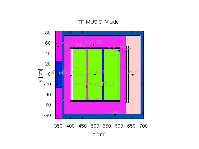
TP-MUSIC IV
The baseline version of the MUSIC simulation considers following and simulates ONLY a signal from the proportional counters (ICs will not be needed for carbon projectiles, PCs measure up to around Q=30 (Sfienti et al. 2003)): Storing structure for each event: 4x2 sensitive regions represent the charge collection regions of the proportional chambers. In these regions we store for each track: entrance and exit point, and ED. It is assumed for the moment that the MUSIC proportional chambers manage to resolve all multiple hits, so for each passing hadron in a sensitive region we compute:- an amplitude \propto released charge in sensitive region
- y-pos (height) (given by mean of track entrance and exit point)
- a signal arrival time (given by TOF from trigger signal to sensitive
- some digitalisation and possibility for adding resolutions and
- the energy deposit dE (or the directly the created ion pairs =dE/W)
- the position coordinates of the energy deposit weighted by dE and their squares.
- the correct fluctuations of created electron-ion pairs should be predicted by FLUKA.
- AMPLITUDE (\propto Q^2): we assume that all the produced charges are collected (times a gain and detector efficiency parameter (*1) and a random Gaussian (*2) for avalanche effects, etc) in the PC column. There is no pulse shape reproduction.
- POSITION information in x (drift time) and y (charge division technique):
- x: drift velocity (*3) and time offset relative to trigger (*4) together with the mean position in x from paragraph 2 will give the x coordinate (with random Gaussian (*5) for diffusion effects, etc).
- y: mean position in y from paragraph 2 will yield directly the y coordinate (with random Gaussian (*6) for diffusion effects, etc).
- There is also no pulse shape reproduction.
- The parameters (*1) - (*6) are directly determined from MUSIC calibration measurements (and can be set for the beginning to dummy values or adapted to older MUSIC calibrations).
- The charge collection efficiency could be set dependent to the distance in which the charge is produced.
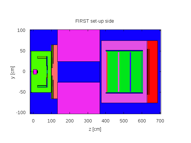
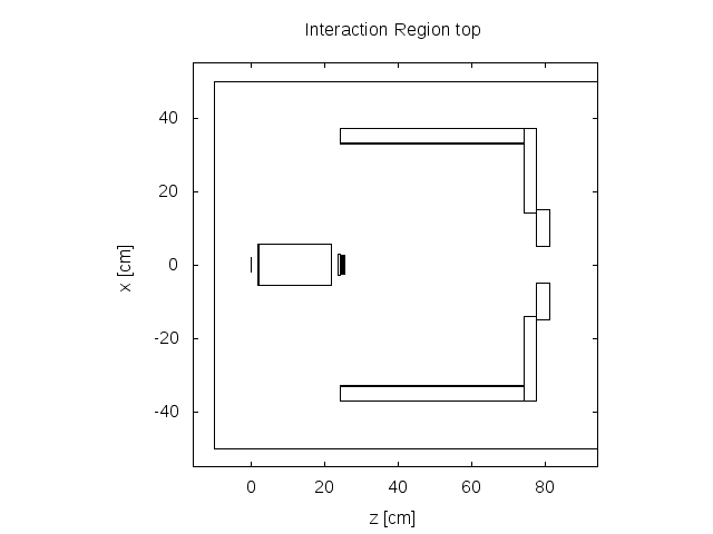
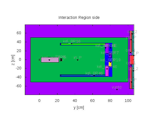
Geometry of the Simulation
- FIRST set-up top view:
- FIRST set-up side view:
- Interaction Region top:
- Interaction Region side:
- MIMOSA 26 top view:
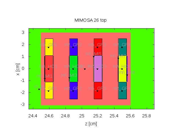
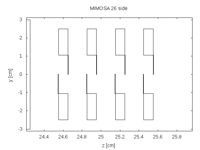
- MIMOSA 26 side view:
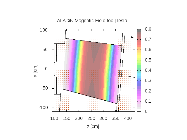
- ALADiN top view:
- ALADiN side view:

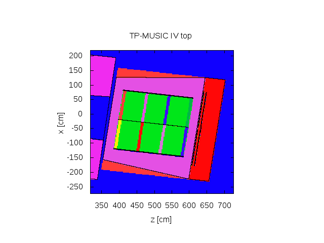
- MUSIC top view:
- MUSIC side view:
- Onion veto detector top view:
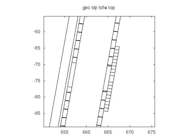
- Onion veto detector top view:
- ALADiN set-up: MUSIC PC numbering scheme
 --------------------------
 |         TOF-Wall       |
 --------------------------

 --------------------------
 |   3                7   |
 |                        |
 |   2                6   |
 |         MUSIC          |
 |   1                5   |
 |                        |
 |   0                4   |
 --------------------------

 -------------------------
 |         ALADiN        |
 -------------------------
            ^
            |z
            |
     x      |
    <-------
-- TillBoehlen - 14 Apr 2011


| I | Attachment | Action | Size | Date | Who | Comment |
|---|---|---|---|---|---|---|
| |
AnaTEST.py.txt | manage | 5 K | 2011-03-13 - 14:33 | UnknownUser | Example script reading the simulation root-file with pyROOT |
| |
FIRSTlogo_2.png | manage | 16 K | 2011-03-31 - 15:46 | UnknownUser | FIRST Experiment long |
| |
MC_Evt1k_test.root | manage | 2 MB | 2011-03-13 - 14:47 | UnknownUser | MC_Evt1k_test.root |
| |
MC_ID039_Evt1k.out | manage | 1 MB | 2011-04-01 - 00:36 | UnknownUser | MC_ID039_Evt1k.out |
| |
MC_ID039_Evt1k.root | manage | 2 MB | 2011-04-01 - 00:21 | UnknownUser | MC_ID039_Evt1k |
| |
geo_AL_side.png | manage | 7 K | 2011-04-01 - 00:53 | UnknownUser | ALADiN side view |
| |
geo_AL_top.png | manage | 9 K | 2011-04-01 - 00:52 | UnknownUser | ALADiN top view |
| |
geo_IR_side.png | manage | 8 K | 2011-03-31 - 15:19 | UnknownUser | Interaction Region side |
| |
geo_IR_top.png | manage | 4 K | 2011-03-31 - 15:18 | UnknownUser | Interaction Region top |
| |
geo_MI_side.png | manage | 4 K | 2011-03-31 - 15:42 | UnknownUser | MIMOSA 26 side view |
| |
geo_MI_top.png | manage | 8 K | 2011-03-31 - 15:41 | UnknownUser | MIMOSA 26 top view |
| |
geo_MU_side.png | manage | 6 K | 2011-03-31 - 15:15 | UnknownUser | MUSIC side view |
| |
geo_MU_top.png | manage | 6 K | 2011-03-31 - 15:14 | UnknownUser | MUSIC top view |
| |
geo_STP_side_colour.png | manage | 3 K | 2011-03-31 - 15:26 | UnknownUser | FIRST set-up side view |
| |
geo_STP_top.png | manage | 6 K | 2011-04-13 - 21:54 | UnknownUser | FIRST set-up top view with beam |
| |
geo_stp_tofw_topOnion.png | manage | 6 K | 2011-03-31 - 15:33 | UnknownUser | Onion veto top view |
| |
svncomment.txt | manage | 15 K | 2012-07-30 - 18:55 | UnknownUser | Simulation log |
Edit | Attach | Print version | History: r33 < r32 < r31 < r30 | Backlinks | View wiki text | Edit wiki text | More topic actions
Topic revision: r33 - 2012-10-30, AlessioSarti
- This page was cached on 2024-04-25 - 04:28.
- User Reference
- BeginnersStartHere
- EditingShorthand
- Macros
- MacrosQuickReference
- FormattedSearch
- QuerySearch
- DocumentGraphics
- SkinBrowser
- InstalledPlugins
- Admin Maintenance
- Reference Manual
- AdminToolsCategory
- InterWikis
- ManagingWebs
- SiteTools
- DefaultPreferences
- WebPreferences
- Categories
Ideas, requests, problems regarding GSI Wiki? Send feedback | Legal notice | Privacy Policy (german)